After this interlude, let us see an example! We will create some data with the following gnuplot script:
reset
a=1.0; b=1.0; c=1.0
f(x) = a*exp(-(x-b)*(x-b)/c/c)
set table 'restrict.dat'
plot [-2:4] f(x)+0.1*(rand(0)-0.5)
unset table
We take a Gaussian, with some noise added to it. Naturally, we would like to fit a Gaussian to this data, and in particular, f(x). But what, if our model is such that 'a' must be in the range [1.1:2], 'b' must be in the range [0.1:0.9], and 'c' must be in the range [0.5:1.5]? We just use in our fit, instead of f(x), another function, g(x), say, of the form
g(x) = A(a)*exp(-(x-B(b))*(x-B(b))/C(c)/C(c))where A(a), B(b), and C(c) take care of our restrictions. These functions are somewhat arbitrary, but for better or worse, I will take the following three arcus tangents
# Restrict a to the range of [1.1:2]
A(x) = (2-1.1)/pi*(atan(x)+pi/2)+1.1

# Restrict b to the range of [0.1:0.9]
B(x) = (0.9-0.1)/pi*(atan(x)+pi/2)+0.1

# Restrict c to the range of [0.5:1.5]
C(x) = (1.5-0.5)/pi*(atan(x)+pi/2)+0.5
which would look like this

The point here is that as x runs from negative infinity to positive infinity, A(x) runs between 1.1, and 2.0, and likewise for B(x), and C(x). Then the fit goes on as it would normally. Our script is, thus, the following in its full glory:
# Restrict a to the range of [1.1:2]
A(x) = (2-1.1)/pi*(atan(x)+pi/2)+1.1

# Restrict b to the range of [0.1:0.9]
B(x) = (0.9-0.1)/pi*(atan(x)+pi/2)+0.1

# Restrict c to the range of [0.5:1.5]
C(x) = (1.5-0.5)/pi*(atan(x)+pi/2)+0.5

a=0.0
b=0.5
c=0.9
fit f(x) 'restrict.dat' via a, b, c

g(x) = A(aa)*exp(-(x-B(bb))*(x-B(bb))/C(cc)/C(cc))
aa=1.5
bb=0.5
cc=0.9
fit g(x) 'restrict.dat' via aa, bb, cc

plot f(x), g(x), 'restrict.dat' w p pt 6
and it produces the following graph:
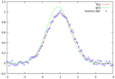
At this point, we should not forget, that what we are interested in is not the value of 'aa', 'bb', or 'cc', but the value of 'a', 'b', and 'c'. This means that what we have to take is
A(aa), B(bb), and C(cc). If you print the values of 'a', 'b', and 'c' from the fit to f(x), the value of 'aa', 'bb', and 'cc', and the value of A(aa), B(bb), and C(cc), we get the following results
gnuplot> pr a, b, c
0.984221984191135 0.996600824504231 1.00765240463672

gnuplot> pr aa, bb, cc
-3442408.91578921 1443864.45093385 -0.201236322474146

gnuplot> pr A(aa), B(bb), C(cc)
1.10000008322047 0.899999823634477 0.936788734177637
Obviously, the second print does not make too much sense, we have to compare the last one to the first one. We can here see that we got values in the ranges [1.1:2], [0.1:0.9], and [0.5:1.5], as we wanted to.
This comment has been removed by the author.
ReplyDeleteTerrificaly interesting post, dear Gnuplotter.
ReplyDeleteIn the past I often switched to ROOT when I had to fit something exactly because of this (in my opinion) huge lack gnuplot has. I was always asking myself "Am I the only person on earth with the necessity of putting constraints on the fitting parameters? Isn't it this feature useful enough to deserve to be implemented directly in the code without having to use such tricks?"
I would be curious to hear what you think.
Cheers
Hello Enrico,
ReplyDeleteWhile I agree with you in principle, I have the feeling that there would be problems with the implementation. The difficulty is that the nature of the most effective restriction scheme would depend on the nature of your problem, and it would be quite hard to come up with a protocol that works in all cases. However, the method that I outlined above is rather straightforward (it needs some handwork, I admit), and flexible. After all, it took only one extra line of code for each variable to achieve what I wanted. I believe, this inconvenience is just not worth the trouble of the implementation.
Cheers,
Zoltán
This comment has been removed by the author.
ReplyDeleteHi Zoltán,
ReplyDeleteSorry for the late reply, I just read your answer.
On one side I agree with you, the implementation you propose is quite straightforward. On the other side, it's still adding a complication that could be avoided.
Then something else: the sensitivity (and sensibility!) of the fit at the extreme boundaries is somehow compromised, don't you think so? A small variation of A(x) (in your example) when A(x) is near 1.1 or 2 reflects in a huge variation on aa, don't you think this could be a problem during the fit procedure? I admit my thoughts are not supported by any theory, just worry and some experience: when the initial factors are near the boundaries, it's sometime difficult to get them out of there.
Cheers,
Enrico
PS sorry for the deleted posts, despite the use of the preview I always find some errors too late.
Very nice, Zoltan. I'm trying to fit some experimental data and needed to constrain my parameters to be non-negative. Thanks for the guidance.
ReplyDeleteHi Zoltán, I'm in the same situation that John.
ReplyDeleteThank you very much
Wow, this was an elegant way to solve it. Thank you!
ReplyDeleteThanks for the method. However, mapping to a semi-infinite interval would be more tricky. Moreover, error estimation of the fit parameters would require additional error propagation calculations. I think it is totally worth it to implement the restriction tools. Even Calc's and Excel's solver (optimizer) utility have this capability. It's a pity that gnuplot does not.
ReplyDeleteHello Zoltan,
ReplyDeleteAn excellent article from a brilliant site. I hope to apply your method to a bounded problem soon. One sideline query i have is how did you plot A(x),B(x),C(x) with the grid ytics at each bound limit? Some sort of overlaid multiplot?
Regards, Dave
Thanks a lot for sharing this. This is so helpful and good to know this kind of techniques.
ReplyDelete--
Mahfuz
Very useful!
ReplyDelete